Algorithms

Understanding Naïve Bayes Algorithm

Naïve Bayes is a classical machine learning algorithm. By reading this post, you will understand this algorithm and implement a Naïve Bayes classifier for classifying the target customer of an ad. by the features of the customer.

Ex10si0n Yan

Feb 14, 2023 • 6 min read

Naïve Bayes Algorithm, mainly refers Multinomial Naïve Bayes Classifier, is a machine learning algorithm for classification. It mathematically based on the Bayes Theorem:

$$P(\text{class}|\text{feature}) = \frac{P(\text{feature}|\text{class})P(\text{class})}{P(\text{feature})}$$

It is easy to prove based on some prior knowledge on Joint probability

$$P(A\cap B)=P(A|B) \cdot P(B)$$

$$P(A\cap B)=P(B|A) \cdot P(A)$$

Hence, we can connect these two formula via $P(A\cap B)$

$$P(A|B) \cdot P(B) = P(B|A) \cdot P(A)$$

Divide both side with $P(B)$,

$$P(A|B) = \frac{P(B|A) \cdot P(A)}{P(B)}$$

Bayes Theorem

Here is an exercise on Wikipedia: Drug testing

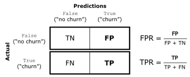
Suppose, a particular test for whether someone has been using cannabis is 90% sensitive, meaning the true positive rate (TPR) = 0.90. Therefore, it leads to 90% true positive results (correct identification of drug use) for cannabis users.

The test is also 80% specific, meaning true negative rate (TNR) = 0.80. Therefore, the test correctly identifies 80% of non-use for non-users, but also generates 20% false positives, or false positive rate (FPR) = 0.20, for non-users.

Assuming 0.05 prevalence, meaning 5% of people use cannabis, what is the probability that a random person who tests positive is really a cannabis user?

$$P(pred_T|real_T) = 0.9$$

$$P(pred_T|real_F) = 0.2$$

$$P(real_T) = 0.05$$

find $P(real_T|pred_T) = ?$

$$P(real_T|pred_T) = \frac{P(pred_T|real_T)P(real_T)}{P(pred_T)}$$

$$P(pred_T)=P(pred_T|real_T)*P(real_T)+P(pred_T|real_F)*P(real_F)$$

$$=\frac{0.9*0.05}{0.05*0.9+0.95*0.2}=0.1914893617$$

Classes and Features

The idea here is to find a class (or say classify) of given features, where class refers to prediction result and features refers all attributes for a specific $X$.

Note that we let $X_i$ be monthly income, martial status of a person, or frequencies of some words in an email, or number of bedrooms, size, distance from subway of a house (which could determine its renting price).

Besides, we could let $y$ be a result corresponding to these $X_i$'s, such as monthly income, martial status of a person may infer the willingness of purchasing by an advertisement, frequencies of some words (free, refund, paid, special) could infer the spam email.

Priors

Since we have figured out the $X$ (feature) and $y$ (class), it is clear that we have frequencies of $X$ and $y$ from statistics. Mathematically, they are $P(\text{feature}_i) = \frac{n(\text{feature}_i)}{n(\text{all})} $ and $P(\text{class}) = \frac{n(\text{class})}{n(\text{all})}$. These kind of probabilities are called priors.

According to the Bayes Theorem which mentioned before:

$$P(\text{class}|\text{feature}) = \frac{P(\text{feature}|\text{class})P(\text{class})}{P(\text{feature})}$$

The bridge connects $P(\text{class}|\text{feature})$ and priors are $P(\text{feature}|\text{class})$. But what are they?

Conditional Probability

In Statistics $P(A|B)$ is conditional probability. $P(A|B)$ is the probability of event $A$ given that event $B$ has occurred. For example, let event B as earthquake, and event A as tsunami. $P(\text{tsunami}|\text{earthquake})$ means when an earthquake happens, the probability of happening a tsunami at the same time. Out of common sense, $P(\text{tsunami}|\text{earthquake})$ is lower when the location of earthquake is far from a coast.

Back to the feature-class, $P(\text{class}|\text{feature})$ and $P(\text{feature}|\text{class})$ refer to two different condition, obviously. Let us make the feature-class be:

$A=P(\text{is spam}|\text{free, refund, paid, special})$ means when a email contains these words: free, refund, paid, special; the probability of it is a spam.

$B=P(\text{free, refund, paid, special}|\text{is spam})$ means when a email is spam (we have already know that), the probability of it containing these words: free, refund, paid, special.

Posteriors

From the previous A and B, we know that B can be easily calculated from given data (in machine learning, we always have some lines of data as input of algorithms), which is "empirical".

While A refers the probability of the email is a spam if given data contains free, refund, paid, special. When the system read an email, and get the vocabulary frequency, it could have these situations:

free       contains | not contains
refund     contains | not contains
paid       contains | not contains
special    contains | not contains

There could be $2^4$ possible combinations of the 4 words. For all emails, they must meet one of the combinations of these words. Hence, we can get a True-False attributes set for the 4 words.

For example, (True, True, True, False) indicates that email contains "free", "refund", "paid" but not contains "special". Then we can get two possibilities.

$$C = P(\text{is spam}|\text{free, refund, paid, not special})$$

$$D = P(\text{is not spam}|\text{free, refund, paid, not special})$$

The task, to find out if the email contains free, refund, paid, but not contains special is a spam, could be converted into find $\max(C, D)$. If C is larger, the email is higher likely to be a spam. Then the classifier could tell the probability of the email contains free, refund, paid, but not contains special is a spam (such as 75%).

Integration

The class-feature $P(\text{class}|\text{feature})$ works as classifier, and it is calculated by Bayes Theorem:

$$P(\text{class}|\text{feature}) = \frac{P(\text{feature}|\text{class})P(\text{class})}{P(\text{feature})}$$

The training process could be mathematically converted into calculation by the given formula.

With the aid of following formulas

$$P(\text{f}|\text{c}) = P(\text{f}_1|\text{c}) \times P(\text{f}_2|\text{c}) \times ... \times P(\text{f}_n|\text{c})$$

$$P(\text{f}) = P(\text{f}_1) \times P(\text{f}_2) \times ... \times P(\text{f}_n)$$

We could cumprod each probabilities and get the posteriors easily.

Implementation

The code implements a Naïve Bayes classifier for finding out if a user will purchase from the advertisement from given features: gender, age, estimation salary.

The data could be downloaded from: https://raw.githubusercontent.com/Ex10si0n/machine-learning/main/naive-bayes/data.csv

wget https://raw.githubusercontent.com/Ex10si0n/machine-learning/main/naive-bayes/data.csv

Step 0: Preprocessing

def split_data(data, ratio):
    np.random.shuffle(data)
    train_size = int(len(data) * ratio)
    return data[:train_size], data[train_size:]

def main():
    f = open('data.csv')
    data = np.array(list(csv.reader(f, delimiter=',')))

    # Cut the first row (headers) and first column (id)
    header = data[0, 1:]
    data = data[1:, 1:]

    # Split data into training and testing sets
    train, test = split_data(data, 0.8)

    # Split data into features and labels
    train_x = train[:, :-1]
    train_y = train[:, -1]
    test_x = test[:, :-1]
    test_y = test[:, -1]

    naive_bayes_classify(header, train_x, train_y, test_x[0], test_y[0])

if __name__ == "__main__":
    main()

Step 1: Calculate all of the conditional probabilities

unique_labels = np.unique(train_y)
p_labels = []
for label in unique_labels:
    count = np.count_nonzero(train_y == label)
    p_labels.append(count / len(train_y))

p_features_given_label = []
for label in unique_labels:
    relevant_rows = train_x[train_y == label]
    for feature in range(len(test_x)):
        count = np.count_nonzero(relevant_rows[:, feature] == test_x[feature])
        p = count / len(relevant_rows)
        p_features_given_label.append(p)
        print("P({}|{}) = {}".format(header[feature], 'purchase' if label == '1' else 'not purchase', p))

Step 2: Calculate all of the priors

p_label_given_features = []
for i in range(len(unique_labels)):
    p = p_labels[i]
    for j in range(len(test_x)):
        p *= p_features_given_label[i * len(test_x) + j]
        print("P({}|{}) = {}".format('purchase' if unique_labels[i] == '1' else 'not purchase', header[j], p))
    p_label_given_features.append(p)

Step 3: Applying the Bayes Theorem

print("P(purchase|{}) = {}".format(test_x, p_label_given_features[0]))
print("P(not purchase|{}) = {}".format(test_x, p_label_given_features[1]))
print("Predicted Label:", 'purchase' if unique_labels[np.argmax(p_label_given_features)] == '1' else 'not purchase')

Result:

========= Conditions =========
P(Gender|not purchase) = 0.5
P(Age|not purchase) = 0.04411764705882353
P(EstimatedSalary|not purchase) = 0.024509803921568627
P(Gender|purchase) = 0.5344827586206896
P(Age|purchase) = 0.017241379310344827
P(EstimatedSalary|purchase) = 0.0

========= Priors =========
P(not purchase|Gender) = 0.31875
P(not purchase|Age) = 0.0140625
P(not purchase|EstimatedSalary) = 0.00034466911764705885
P(purchase|Gender) = 0.19374999999999998
P(purchase|Age) = 0.00334051724137931
P(purchase|EstimatedSalary) = 0.0

========= Results =========
P(purchase|['Female' '27' '57000']) = 0.00034466911764705885
P(not purchase|['Female' '27' '57000']) = 0.0
Predicted Label: not purchase
Actual Label: not purchase

View full code here:

Conclusion

Naïve Bayes is a fast and simple algorithm that requires a little training data, making it suitable for large datasets or data with limited labeled examples. It also has the advantage of being able to handle multiple classes, making it a popular choice for text classification and spam filtering.

In conclusion, Naïve Bayes is a simple yet powerful algorithm that is widely used in many real-world applications. Despite its "naïve" assumption of independent features, it has proven to be a reliable method for classification in many scenarios.