Introduction

In the past 10 years, the best-performing artificial-intelligence systems — such as the speech recognizers on smartphones or Google’s latest automatic translator — have resulted from a technique called “Deep Learning.”

Deep learning is in fact a new name for an approach to artificial intelligence called neural networks, which have been going in and out of fashion for more than 70 years. Neural networks were first proposed in 1944 by Warren McCullough and Walter Pitts.

Neural network is an interconnected group of nodes, inspired by a simplification of neurons in a brain. It works similarly to the human brain’s neural network. A “neuron” in a neural network is a mathematical function that collects and classifies information according to a specific architecture. The network bears a strong resemblance to statistical methods such as curve fitting and regression analysis.

In this post, we’ll understand how neural networks work while implementing one from scratch in Python.

Perquisite: already learned one of the Data Science Utilities numpy from 25 exercises to get familiar with Numpy.

DS Utilities: Numpy | Python-ML

Logo

Since you have learned it yet, we have enough knowledge to learn how to implement a Neural Network only using numpy. This lecture is inspired from VictorZhou's Blog.

victorzhou.com

Software Engineer. I blog about web development, machine learning, and more topics.

Victor Zhou

Neuron in Biology

In field of study in Neuroscience and Biology, scientists have already built the model of a Neuron (Nerve cell) in creatures brains. a Neuron is illustrated as follow:

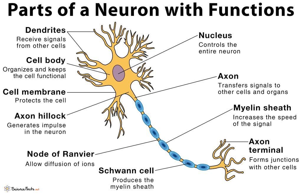
Now focus on these 3 components:

• Dendrites: Receive signals from other cells.
• Axon hillock: Generates impulse in the neuron.
• Axon terminal: Forms junctions with other cells.

At the Dendrites, neurotransmitters are released, triggering nerve impulse in neighboring neurons. When the neighboring nerve cell(s) receives a specific impulse, the cell body will be activated and transmit electronic signal through the Axon by the effect of exchanging electrons with Na+/K+-ATPase.

Remember, a neuron is always connected to many other neighboring neurons in the Axon terminal side, meanwhile; a neuron can also receive impluse from previous neurons in the Dendrites side. As an example:

Metaphor: Interpersonal Relationship

There is a boy called Tom, he has a simple interpersonal relationship described as the following picture:

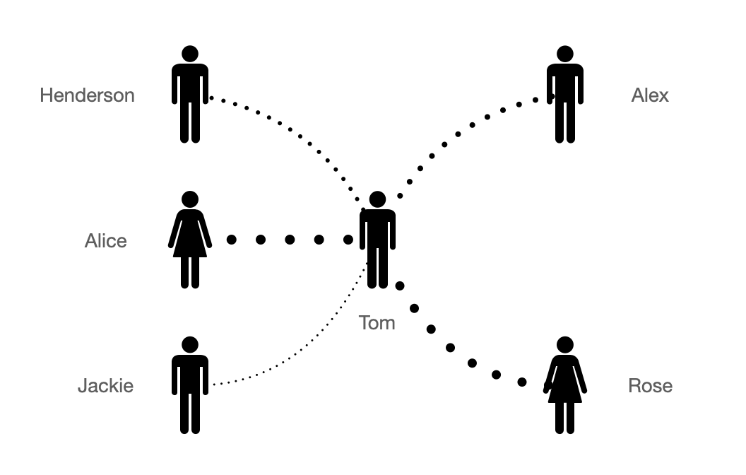
Henderson and Alice are Tom's good friends while Jackie is Tom's colleague, it is clear that Tom will arrange higher priorities with affairs from Henderson and Alice, and a lower priorities to Jackie. Relatively, Rose regards Tom as good friend so when Tom tells Rose something, she will be more active than Alex in helping Tom.

Years later, with the co-operation with Jackie, Tom and Jackie will be more close and be good friend, they talk to each other everything. So the connection between Jackie and Tom will the stronger, and Tom will arrange higher priorities to Jackie.

Tom also have a threshold on which kind of people he can help and which kind of people he will reject. Meanwhile, the threshold is always changing for each people. Maybe someday, Tom and Alice have not communicated with each other for several month, and Tom will regards Alice not as close as before, so he will adjust the threshold.

Back to neurons, the relationships is similar. With multiple neurons work as the interpersonal relationship, they are forming a network like social networks. And that is why our brains can think, action and create as well as having emotion.

Neurons

Now let us model the working principle of neurons with programming language. Image a function which can take two input parameters as x1, x2 and returns output y. In Python code:

def f(x1, x2):
  ...
  return y

he implementation ... of the function are in three steps:

1. Calculate weighted x1 and x2
2. Add a bias to adjust the weighted value from step 1
3. Determine in what extents we can accept the value from step 2

To illustrate the implementation, we have:

Note that, weights w1, w2 and bias b can be changed during the time. And accept_level can be considered as the threshold to determine how much y will be.

This function works as a neuron which we have introduced before. There will be many neurons interconnected as a network.

In this example, we regards:

• x1, x2 as the output from the previous neuron.
• y as the output of current function.
• activation() is the activation function which used to turn an unbounded input into an output that has a nice, predictable form.

Activation Function

Consider a classification problem: You are taking a test at school, if your test mark is lower than 50, your mama will beat you when you back home. Otherwise, she will treate you a delicious dinner

we can consider

• x = your mark - 50
• when x is positive, you will have a delicious dinner
• when x is negative, you will be beaten by mama

That is the following diagram:

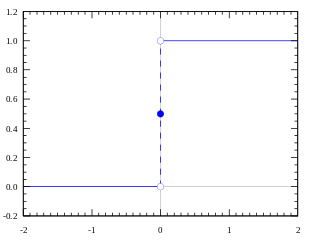
• y = 1 means you have dinner
• y = 0 means you got beat

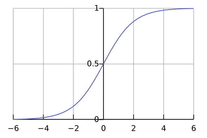
But it is not fair for your score is around 50, which means only 1 mark difference will make you be in two results. Why not make the line smooth, and when you got whatever 49 or 51 your mama will just say: It's okay, be better next time.

Sigmoid activation function works well in this scenario:

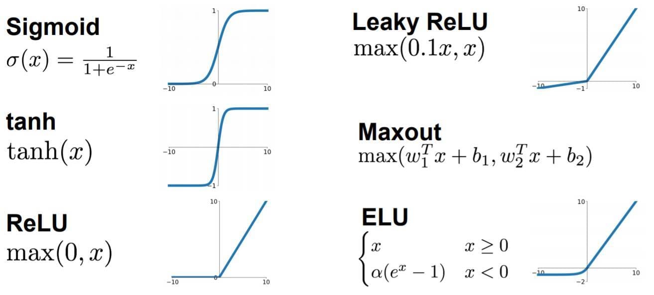
Back to the activation function, actually there are many kinds of functions and they work well in different senarios.

Coding Neuron

In order to manage the relationship well. We can make a Neuron class to struturalize a neuron unit. In which, the feedforward() function is the previous f(x1, x2). And inner implementation of the f() function changes in order to get vector input inputs, so it will be np.dot() instead of w1 * x1 + w2 * x2. If you are not familiar with dot product, please refer: Dot product in Wiki.

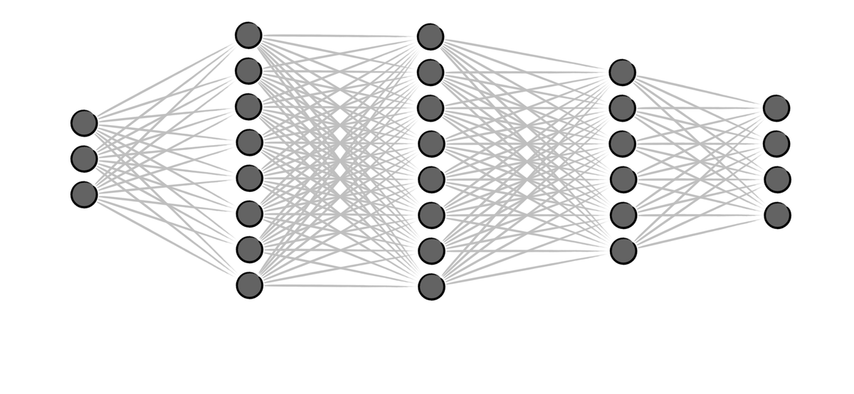
Neuron Network

A neural network is nothing more than a bunch of neurons connected together. Here’s what a simple neural network might look like:

This network has 2 inputs, a hidden layer with 2 neurons (h1 and h2), and an output layer with 1 neuron (o1). Notice that the inputs for o1 are the outputs from h1 and h2 - that’s what makes this a network. In addition, h1, h2, o1 are all instances of class Neuron.

A hidden layer is any layer between the input (first) layer and output (last) layer. There can be multiple hidden layers!

Feed-forward

We assumed that all of the Neurons (h1, h2, o1) have the same weights w = [0, 1] and bias b = 0. Then if we pass input x1 = 2, x2 = 3 into the network. We have:

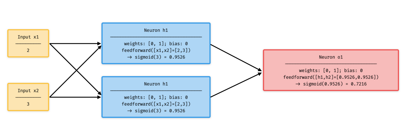
A neural network can have any number of layers with any number of neurons in those layers. The basic idea stays the same: feed the input(s) forward through the neurons in the network to get the output(s) at the end.

Coding Feed-forward

Here is the code implementing the previous feedforward process of our neural network.

We got the same result compared with the illustrated diagram in Feed-Forward section.

Training a Neural Network (Part 1)

Let’s train our network to predict someone’s gender given their weight and height:

We’ll represent Male with a 0 and Female with a 1, and we’ll also shift the data to make it easier to use:

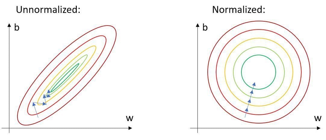
I arbitrarily chose the shift amounts (135 and 66) to make the numbers look nice. Normally, you’d shift by the mean.

The process making data more easier to use follows the methodology of Normalization.

Linear Regression

Before we start the training process, let's have a quick review on Linear Regression:

Consider a plot of scatter points (x_i, y_i)which repectively represents (rental price, house area). As common sense, the x and y has a positive correlation. We can plug in each x_i and y_i into the formula of Least Squares Method:

Where m called correlation coefficient and the equation of the regression line is:

For linear regression, we can get the equation easily. But for Multiple Linear Regression with many parameter x's, it will become complex.

And we know that, to predict the house rental price, we cannot consider only one factor which is house area. We should also take Location, Number of Bedrooms, Appliances and Other Amenities, Curb Appeal and Condition and even if the house is Allowing Pets. Then the regression process will be further more complex. So we should determine another method to optimize the calculating time.

Loss

Let us have a look at a common component of regression. We know that any of the avaliable regression cannot pass through all of the points of (x, y). There may be many points below line or on the upwards. So the Loss is defined to describe the regression's level of inaccurate.

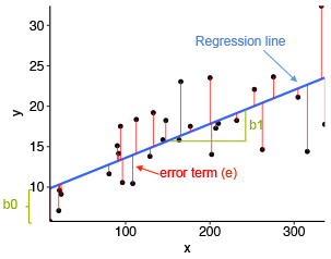
The red lines describe absolute value of y_accurate - y_predict. As an example, we use the mean squared error (MSE) loss:

Turn this formula to Python code is straightforward:

Gradient Descent

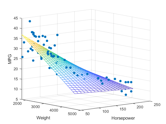
Assume that The z axis (height) is the loss, x and y are the correlation coeffiecients of a Multiple Linear Regression. There may be a 3D plot as follows.

To get the optimized regression effect. We should determine the lowest z on the plot and the coefficients are the corresponding x and y. If we can get this plot, we can easily find where is the lowest z.

Unfortunately, in practice, like playing a open-world game. It always has fog covering the unvisited area. We only have the information of starting up point, and we need to try each direction to explore.

But, at least, we may know where to go like: try not going to the desert at first.

Same as calculating the optimized correlation coefficient. Although we do not know all of the map, we can refer to the gradient where we are standing on. We can refer gradient as slope in higher dimension plot.

Positive gradient: go Left
Negative gradient: go Right

Training a Neural Network (Part 2)

We now have a clear goal: minimize the loss of the neural network. We know we can change the network’s weights and biases (each weights and bias in a Neuron) to influence its predictions, but how do we do so in a way that decreases loss?

To think about loss is as a function of weights and biases. Let’s label each weight and bias in our network:

Then the loss of the whole Network are determined by weight and bias in each Neurons:

Backpropagation

If we want to make w1 a little bit higher or lower, how would Loss change? The loss is the function of every weights and biases. So we need to calculate the gradient of the 2D slice (x, y) = (w1, L) of a 9D plot is partial derivative.

$$
\text{determine}: \frac{\partial{L}}{\partial w_i}
$$

$$
\frac{\partial L}{\partial{w_i}} = \frac{\partial L}{\partial y_{pred}} \times \frac{\partial y_{partial}}{\partial{w_i}}
$$

$$
= \frac{\partial L}{\partial y_{pred}} \times \frac{\partial y_{pred}}{\partial h_1} \times \frac{\partial h_1}{\partial w_1}
$$

$$
\frac{\partial L}{\partial y_{pred}} = \frac{\partial \frac{\sum\limits_{i=0}^{n} (y_i - y_{pred})}{n}}{\partial y_{pred}}
$$

$$
\frac{\partial y_{pred}}{\partial h_1} = \frac{\partial \text{sigmoid}(w_5 h_1 + w_6 h_2 + b_3)}{\partial h_1} = w_5 \text{sigmoid}'(w_5 h_1 + w_6 h_2 + b_3)
$$

$$
\frac{\partial h_1}{\partial w_1} = \frac{\partial \text{sigmoid}(w_1 x_1 + w_2 x_2 + b_1)}{\partial w_1} = x_1 \text{sigmoid}'(w_1 x_1 + w_2 x_2 + b_1)
$$

$$
\text{sigmoid}(x) = \frac{1}{1 + e^{-x}}
$$

This system of calculating partial derivatives by working backwards is known as backpropagation, or “backprop”.

Optimizer

We have all the tools we need to train a neural network now! We’ll use an optimization algorithm called stochastic gradient descent (SGD) that tells us how to change our weights and biases to minimize loss. It’s basically just this update equation:

η is a constant called the learning rate that controls how fast we train. We use η times ∂L/∂w1 to adjusting w1:

• if ∂L/∂w1 is positive, according to SGD w1 will decrease, L = f(w1) is decrescent function, L will decrease
• if ∂L/∂w1 is negative, according to SGD, w1 will increase, L = f(w1) is increasing function, L will decrease

If we do this for every weight and bias in the network, the loss will slowly decrease and our network will improve.

Our training process will look like this:

1. Choose one sample from our dataset. This is what makes it stochasticgradient descent - we only operate on one sample at a time.
2. Calculate all the partial derivatives of loss (example using ∂L/∂w1 , but we need to find all w and b) with respect to weights or biases
3. Use the update equation to update each weight and bias.
4. Go back to step 1.

Implementing with Python is, we refer each w and b is random:

Then we input some train data from the following table.

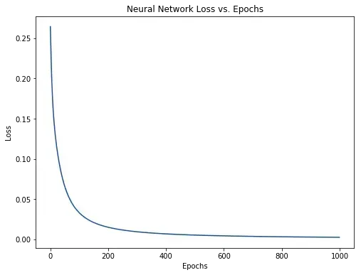
Our loss steadily decreases as the network learns:

We can now use the network to predict genders:

Try your personal data:

Conclusion

You made it! A quick review of what we did:

• Introduced neurons, the building blocks of neural networks.
• Used the sigmoid activation function in our neurons.
• Saw that neural networks are just neurons connected together.
• Created a dataset with Weight and Height as inputs (or features) and Gender as the output (or label).
• Learned about loss functions and the mean squared error (MSE) loss.
• Realized that training a network is just minimizing its loss.
• Used backpropagation to calculate partial derivatives.
• Used stochastic gradient descent (SGD) to train our network.

Thanks for reading!