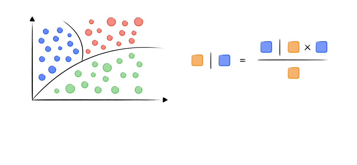
Naïve Bayes Algorithm, mainly refers Multinomial Naïve Bayes Classifier, is a machine learning algorithm for classification. It mathematically based on the Bayes Theorem:

$$​​P(\text{class}|\text{feature}) = \frac{P(\text{feature}|\text{class})P(\text{class})}{P(\text{feature})}$$

It is easy to prove based on some prior knowledge on Joint probability

$$P(A\cap B)=P(A|B) \cdot P(B)$$

$$P(A\cap B)=P(B|A) \cdot P(A)$$

Hence, we can connect these two formula via $P(A\cap B)$

$$P(A|B) \cdot P(B) = P(B|A) \cdot P(A)$$

Divide both side with $P(B)$,

$$P(A|B) = \frac{P(B|A) \cdot P(A)}{P(B)}$$

Bayes Theorem

Here is an exercise on Wikipedia: Drug testing

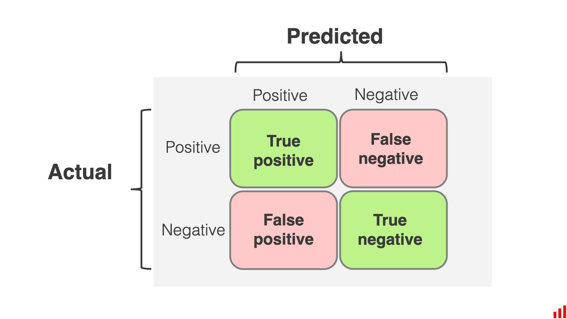
Suppose, a particular test for whether someone has been using cannabis is 90% sensitive, meaning the true positive rate (TPR) = 0.90. Therefore, it leads to 90% true positive results (correct identification of drug use) for cannabis users.

The test is also 80% specific, meaning true negative rate (TNR) = 0.80. Therefore, the test correctly identifies 80% of non-use for non-users, but also generates 20% false positives, or false positive rate (FPR) = 0.20, for non-users.

Assuming 0.05 prevalence, meaning 5% of people use cannabis, what is the probability that a random person who tests positive is really a cannabis user?

$$P(pred_T|real_T) = 0.9$$

$$P(pred_T|real_F) = 0.2$$

$$P(real_T) = 0.05$$

find $P(real_T|pred_T) = ?$

$$P(real_T|pred_T) = \frac{P(pred_T|real_T)P(real_T)}{P(pred_T)}$$

$$P(pred_T)=P(pred_T|real_T)*P(real_T)+P(pred_T|real_F)*P(real_F)$$

$$=\frac{0.9*0.05}{0.05*0.9+0.95*0.2}=0.1914893617$$

Classes and Features

The idea here is to find a class (or say classify) of given features, where class refers to prediction result and features refers all attributes for a specific $X$.

Note that we let $X_i$ be monthly income, martial status of a person, or frequencies of some words in an email, or number of bedrooms, size, distance from subway of a house (which could determine its renting price).

Besides, we could let $y$ be a result corresponding to these $X_i$'s, such as monthly income, martial status of a person may infer the willingness of purchasing by an advertisement, frequencies of some words (free, refund, paid, special) could infer the spam email.

Priors

Since we have figured out the $X$ (feature) and $y$ (class), it is clear that we have frequencies of $X$ and $y$ from statistics. Mathematically, they are $P(\text{feature}_i) = \frac{n(\text{feature}_i)}{n(\text{all})} $ and $P(\text{class}) = \frac{n(\text{class})}{n(\text{all})}$. These kind of probabilities are called priors.

According to the Bayes Theorem which mentioned before:

$$​​P(\text{class}|\text{feature}) = \frac{P(\text{feature}|\text{class})P(\text{class})}{P(\text{feature})}$$

The bridge connects $​​P(\text{class}|\text{feature})$ and priors are $P(\text{feature}|\text{class})$. But what are they?

Conditional Probability

In Statistics $P(A|B)$ is conditional probability. $P(A|B)$ is the probability of event $A$ given that event $B$ has occurred. For example, let event B as earthquake, and event A as tsunami. $P(\text{tsunami}|\text{earthquake})$ means when an earthquake happens, the probability of happening a tsunami at the same time. Out of common sense, $P(\text{tsunami}|\text{earthquake})$ is lower when the location of earthquake is far from a coast.

Back to the feature-class, $​​P(\text{class}|\text{feature})$ and $P(\text{feature}|\text{class})$ refer to two different condition, obviously. Let us make the feature-class be:

$A=P(\text{is spam}|\text{free, refund, paid, special})$ means when a email contains these words: free, refund, paid, special; the probability of it is a spam.

$B=P(\text{free, refund, paid, special}|\text{is spam})$ means when a email is spam (we have already know that), the probability of it containing these words: free, refund, paid, special.

Posteriors

From the previous A and B, we know that B can be easily calculated from given data (in machine learning, we always have some lines of data as input of algorithms), which is "empirical".

While A refers the probability of the email is a spam if given data contains free, refund, paid, special. When the system read an email, and get the vocabulary frequency, it could have these situations:

free       contains | not contains
refund     contains | not contains
paid       contains | not contains
special    contains | not contains

There could be $2^4$ possible combinations of the 4 words. For all emails, they must meet one of the combinations of these words. Hence, we can get a True-False attributes set for the 4 words.

For example, (True, True, True, False) indicates that email contains "free", "refund", "paid" but not contains "special". Then we can get two possibilities.

$$C = P(\text{is spam}|\text{free, refund, paid, not special})$$

$$D = P(\text{is not spam}|\text{free, refund, paid, not special})$$

The task, to find out if the email contains free, refund, paid, but not contains special is a spam, could be converted into find $\max(C, D)$. If C is larger, the email is higher likely to be a spam. Then the classifier could tell the probability of the email contains free, refund, paid, but not contains special is a spam (such as 75%).

Integration

The class-feature $P(\text{class}|\text{feature})$ works as classifier, and it is calculated by Bayes Theorem:

$$​​P(\text{class}|\text{feature}) = \frac{P(\text{feature}|\text{class})P(\text{class})}{P(\text{feature})}$$

The training process could be mathematically converted into calculation by the given formula.

With the aid of following formulas

$$P(\text{f}|\text{c}) = P(\text{f}_1|\text{c}) \times P(\text{f}_2|\text{c}) \times ... \times P(\text{f}_n|\text{c})$$

$$P(\text{f}) = P(\text{f}_1) \times P(\text{f}_2) \times ... \times P(\text{f}_n)$$

We could cumprod each probabilities and get the posteriors easily.

Implementation

The code implements a Naïve Bayes classifier for finding out if a user will purchase from the advertisement from given features: gender, age, estimation salary.

The data could be downloaded from: https://raw.githubusercontent.com/Ex10si0n/machine-learning/main/naive-bayes/data.csv

wget https://raw.githubusercontent.com/Ex10si0n/machine-learning/main/naive-bayes/data.csv

Data Preprocessing

The provided code reads data from a CSV file, separates the headers and data, splits it into training and testing sets, and further splits them into features and labels.

Calculate all of the conditional probabilities

Calculate all of the priors

Applying the Bayes Theorem

Result

View full code here:

machine-learning/naive-bayes at main · Ex10si0n/machine-learning

Tutorial of Python Machine Learning Implementation on Linux - machine-learning/naive-bayes at main · Ex10si0n/machine-learning

GitHubEx10si0n

Conclusion

Naïve Bayes is a fast and simple algorithm that requires a little training data, making it suitable for large datasets or data with limited labeled examples. It also has the advantage of being able to handle multiple classes, making it a popular choice for text classification and spam filtering.

In conclusion, Naïve Bayes is a simple yet powerful algorithm that is widely used in many real-world applications. Despite its "naïve" assumption of independent features, it has proven to be a reliable method for classification in many scenarios.