Implementing JPEG Image Compression Algorithm using MATLAB

In this tutorial, we will implement a image compression algorithm using MATLAB. JPEG stands for Joint Photographic Experts Group, which was a group of image processing experts that devised a standard for compressing images (ISO).

JPEG Image Compression

The JPEG (or JPG) format is not technically a file format, but rather an image compression standard. The JPEG standard is complex, with various options and color space regulations. However, it was not widely adopted. Simultaneously, a simpler version called JFIF was advocated. This is the image compression algorithm commonly referred to as JPEG compression, and the one we will be discussing in this class. It's worth noting that the file extensions .jpeg and .jpg have persisted, even though the underlying algorithm strictly follows JFIF compression.

The Underlying Assumptions of the JPEG Algorithm

The JPEG algorithm is designed specifically for the human eye. It exploits the following biological properties of human sight:

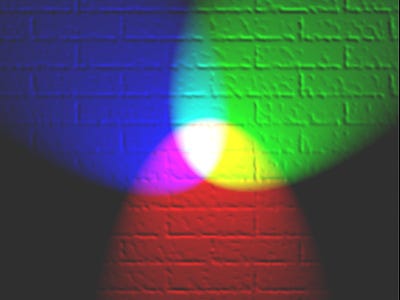
We are more sensitive to the illuminocity of color, rather than the chromatric value of an image
We are not particularly sensitive to high-frequency content in images.

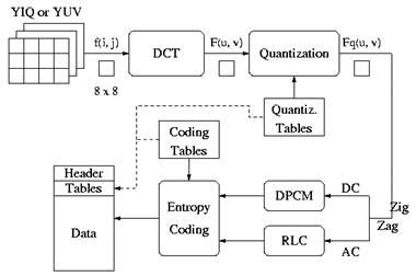
The algorithm can be neatly illustrated in the following diagram:

Matlab Implementation: Encoder

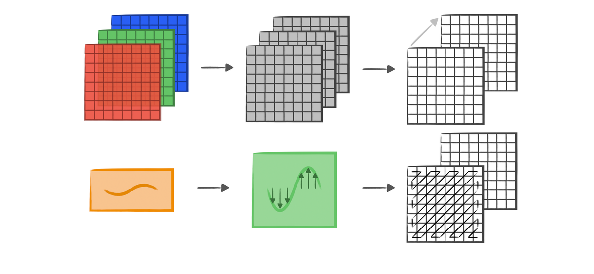
Assume img is the image we have read in. In JPEG compression, all compression processes should be carried on in YCbCr color space. In this color space, Cb is the blue component relative to the green component while Cr is the red component relative to the green component.

Here is the built-in Matlab code for converting the color space.

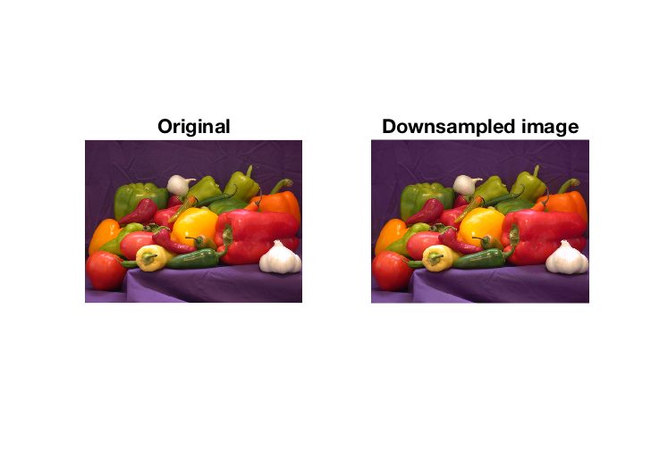
The YCbCr is a more convenient colorspace for image compression because it separates an image's illuminance and chromatic strength. Since our eyes are not particularly sensitive to chrominance, we can "downsample" that. Here, half the amount of "color" and generate the Y_dsp representing downsampled Y. The difference between original and downsampled image is imperceptible, as you can see from the result.

Downsampling, Image from pi.math.cornell.edu

Following the steps, we need to apply the following processes for each 8x8 blocks in the image. Y_dct is the matrix contains frequency domain of original image specifically for every 8x8 block. In another word, we apply discrete cosine transform (DCT) for every 8x8 block and store these 8x8 results matrices into Y_dct.

Then we apply DCT inside the preceding tripe for loop, this process transform the original image from spatial domain to frequency domain:

Quantization is a process in which we take a couple of values in a specific range and turns them into a discrete value. (also called discretization). It is intuitive that after DCT, quantization converts the higher frequency coefficients in the output matrix to 0.

Besides, the intensity of quantization determines the extend of data retaining for the image. Quantization is applied and how much of higher frequency information is lost, and this is the reason why JPEG is a lossy compression.

Since we have got the matrix in frequency domain, we could apply quantization using a quantization table Q.

After quantization, the image has been compressed a lot, however; in order to have a extreme compression, we should consider the potential of compressing the quantized data using entropy coding (i.e. Huffman Coding).

However, since Y_dct now is a 2D matrix, we need to convert it to 1D firstly. Yet, there is many ways of converting 2D array to 1D. Due to the characteristic of "DCTed" array - large numbers always lies on top-left, zig-zag is a better choice.

To implement zig-zag, we could declare a zig-zag table as follows.

This table is designed by the process of zig-zagging, which is illustrated in the following diagram. Zig-zag ensures top-left first, then positive (non-negative) numbers in the generated 1D array should be lies on the staring points.

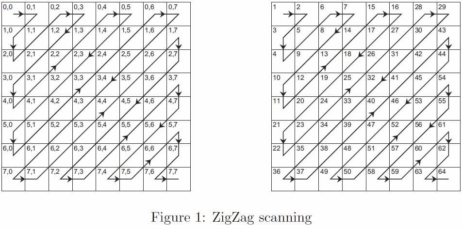
Here is the code for zig-zagging.

Till now, we have turned the 2D Y_dct into Y_lin which represents linear 1D array. To better handling this 1D array, DC and AC are two essential part to be implemented.

DC is the different first digit of Y_lin between the preceding first digit for every adjacent 8x8 blocks. AC is the rest of digits (2, 64) in Y_lin for the current 8x8 block.

AC should be applied with Run Length Encoding (RLE) if you are not familiar with this, please refer: filestore.aqa.org.uk(PDF). The code below is RLE codec.

Hence, we could apply RLE to AC, and append BC, AC to a data payload.

Huffman encoding is a pretty concise and elaborate entropy encoding yields optimal prefix code that is commonly used for lossless data compression. Code for a simple implementation of Huffman encoding in Python could be found at:

Then we could apply built-in Huffman encoding to all payloads all at onces.

Then we could store dict into header and bit_stream as compressed image data, they encapsulate them to a single file. That's it, we have implemented a JPEG encoder (Image to bitstream) now.

Matlab Implementation: Bit stream

In the generated data (say bit stream), it should store some information inside its header, such as, dictionary header_dict used for huffman encoding. Moreover, since AC was applied through RLE, and then we encapsulate it with DC inside a payload. There should be a header for maintaining how long for each payload, in this implementation, we uses header_ac_seperator to store this information. Besides, resolution of orginial image should also be stored because without it we cannot specify the image row-column ratio when rebuilding it, that make sense. Finally, quality coeffeicient should also be stored in the header since it is determined only when encoding.

Matlab Implementation: Decoder

Inversely, to employ JPEG decoder, just inverse these processes. Firstly, after receiving content for bit stream, we apply huffman decoding to it

Then, refering header_ac_seperator, we could re-constructuct each payload [DC AC] which we have mentioned previously.

Then, we applied inverse zig-zag using the same zig-zagging sequence, inverse quatization, and inverse DCT.

We can rebuild each block in the image.

To make the iteration works, some iteration variables should be changed during the loop

Finally, we change the color space from YCbCr to RGB

Run it and have a look.

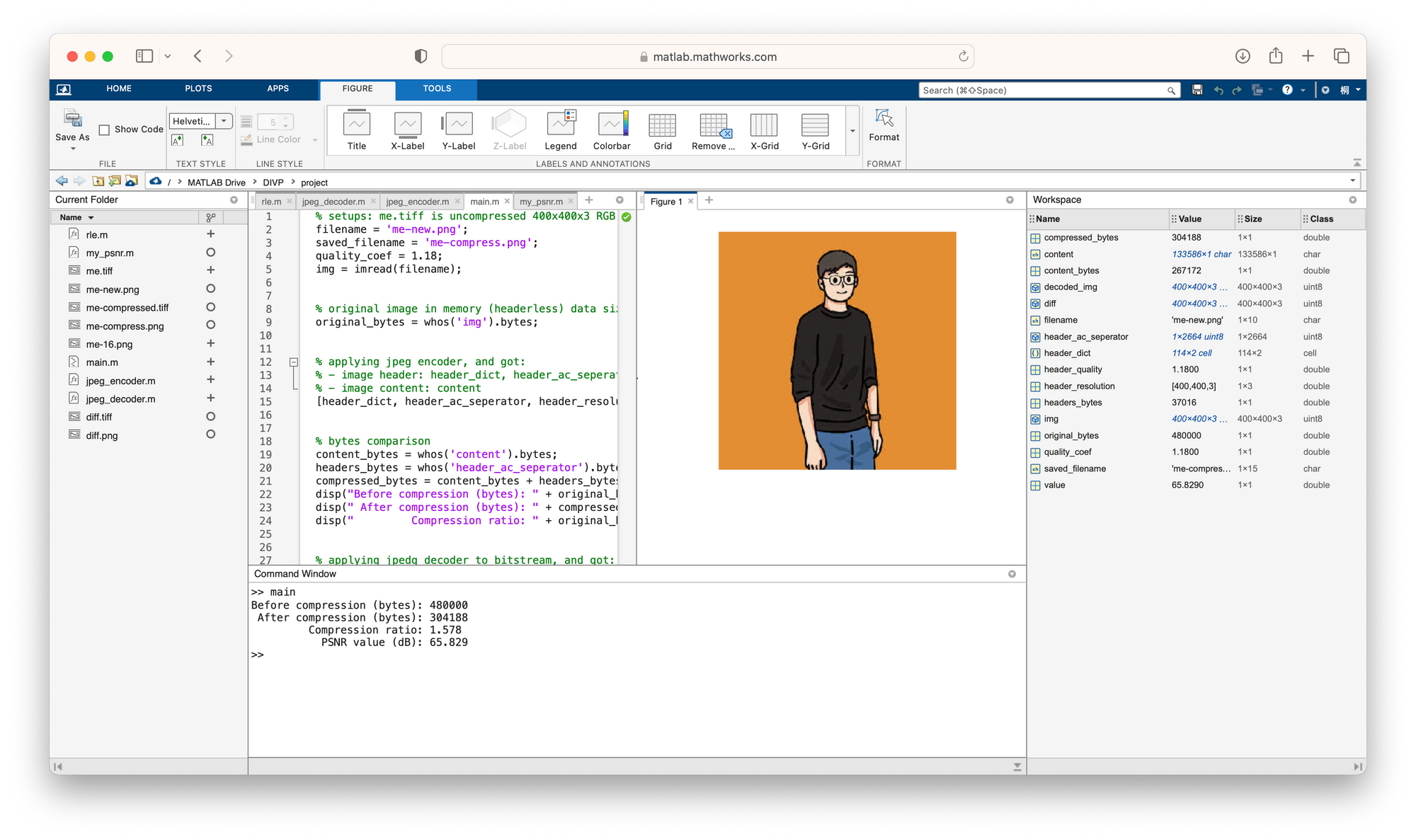
We can see the image compression ratio in comparing original headless image data vs. compressed header and content:

   Compression coefficient: 1.1800
Before compression (bytes): 480000
 After compression (bvtes): 304188
         Compression ratio: 1.5780
           PSNR value (dB): 65.829

Bingo! We have achieved a JPEG decoder now by inversely designing the encoder. Take a look at the decoded compressed image.

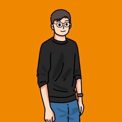
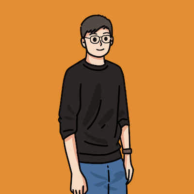
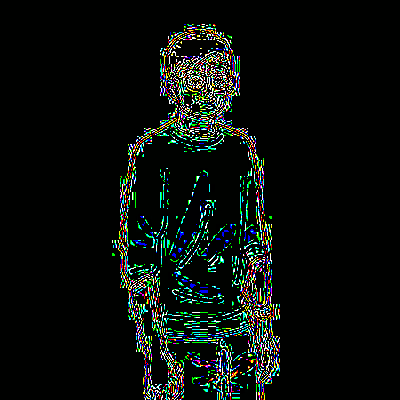
We can see that in the compressed image, pixels on the edges of the guy is quite weird, it is because the mini-block-wise DCT sampling have different rounded value. To compared with the original image, the image different could be calculated by setting threshold as 3.

Now we have visualized the different between original and compressed image.

Conclusion

We have implemented a JPEG codec in this tutorial, now you have learned:

YCbCr color space
Discrete Cosine Transform and Inverse Discrete Cosine Transform (to be added)
JPEG encoding process (image to blocks - DCT - quantization - zigzagging - entropy encoding - encapsulation)
JPEG decoding process (decapsulation - entropy decoding - inverse zigzagging - inverse quantization - iDCT - blocks to image)
Some of the JPEG headers

You can find the code at my Github via the following link: