Forming Vision: How a Conv Neural Network Learns

Implementing Neural Networks from Scratch

In this post, we’ll understand how neural networks work while implementing one from scratch in Python.

Aspires - Ex10si0nEx10si0n

In the previous post, we introduced how a Neural Network learns in aspect of mathematical simulation of neurons. In this post, we will introduce the advanced architecture of neuron networks - Convolution Neural Networks - which, in some aspect, forms a vision that can extract features automatically.

Filtering & Kernels

In the area of Digital Image Processing, it is well-known that there are many kinds of filters to fulfill a specific kind of work, such as border detection, blurring, sharpening, etc.

As an example of applying border detection on a grayscale image, the Sobel and Laplacian Edge Detectors can detect the border (sudden change of pixel values) via the filter, or say kernel, for the Laplacian operator:

$$\begin{bmatrix} -1 & -1 & -1 \\ -1 & 8 & -1 \\ -1 & -1 & -1 \end{bmatrix} $$

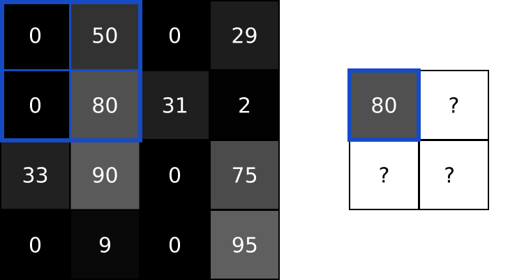
The filter then be applied to the image as sliding window, as shown in the animation below:

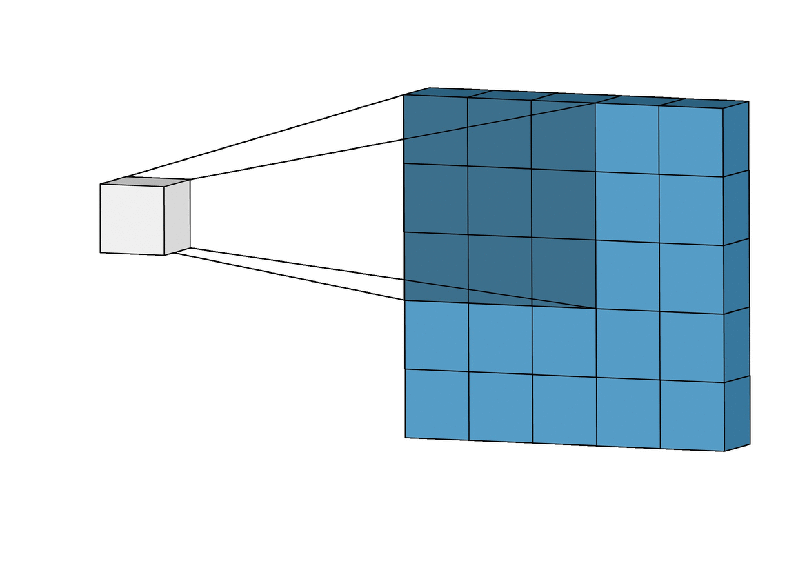
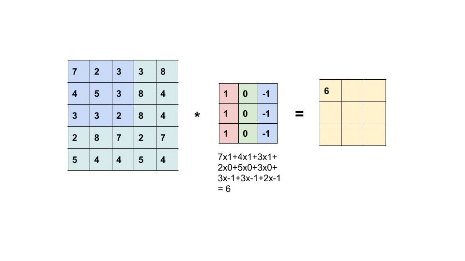
What happens in each filtering (white box in the front) follows the below calculation:

Due to the characteristic of kernel design, borders could be detected as shown in the image below.

Convolution

Image filtering and convolution are two closely related concepts used in image processing, however; they have a slightly difference:

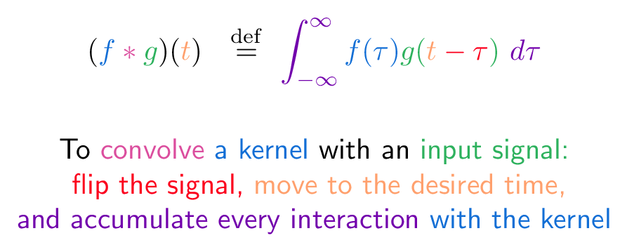
The convolution operation moves the input image to desired time (you can regard it as going cross-wise rather than parallel*, since the term time in signal processing represents time-frequency related to spatial-frequency)

To a better understanding, it doesn't matter to regard convolution as a way of filtering since the key here is to shrink the size of image while retraining its features as much as possible.

Fully Automatic on Parameter Optimizing

By recapping the gradient descent in training a Neural Network, we know that:

• Learning is in fact minimizing the loss automatically
• The loss is determined by data (X), label (y), weights and bias (W, b)
• Data(X), and label(y) cannot be change (usually) since they are ground truth
• The network parameters weights and bias (W, b) can be changed to optimize the performance of that network
• In back-propagation, weights and bias (W, b) are descent by gradient of loss with respect to each weight and bias respectively

Hence, the Neural Net can learn by changing its network parameters, i.e. weights and bias (W, b).

So How to Determine the Kernel?

By the gradient descent, the neural network can learned by updating its parameters. However, the CNN architecture is firstly comes with Convolutional Layers, connected with a Fully Connected Layer, or say deep neural network. Note that the Convolutional Layers contain kernel for each specific layers, the kernel is simply set as a random matrix. The key point is each kernel can be also updated by the gradient descent:

During the training process, each entry of the kernel is updated by calculating the partial derivative of the loss function with respect to that entry of the kernel.

Wow, the kernels can also learn by itself. As different training data, the kernel can be formed to a specific matrix which are relatively optimal to the specific task regardless to classification and segmentation.

Extracting Features and Poolings

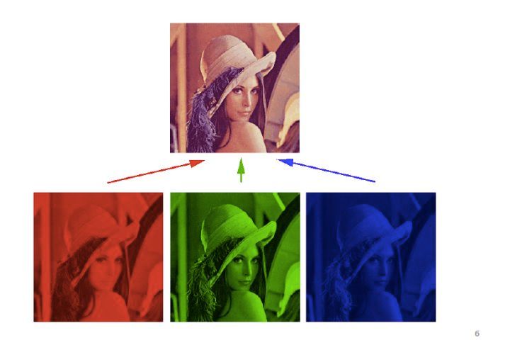
Although CNN can handle the task other than images, we simply use the most classical task - image classification - to illustrate the process. A colored image is usually adopting RGB format, which contains three channels, Red, Green, Blue, respectively. The image of Lena is a classical computer image processing example, the following are the RGB channels, for example, the Red channel have only the magnitude of red color, the lighter pixel the higher magnitude it is. The colored image of Lena is the composition of magnitudes of the three color channels.

For a CNN, to handle the colored image, we usually apply a 3 channel to n channel convlution layer firstly. In the following diagram, each black b0x is a kernel.

To simplified, we set all the kernel to 3x3, hence 26x26 image can be reduced to 24x24 since no image paddings are used.

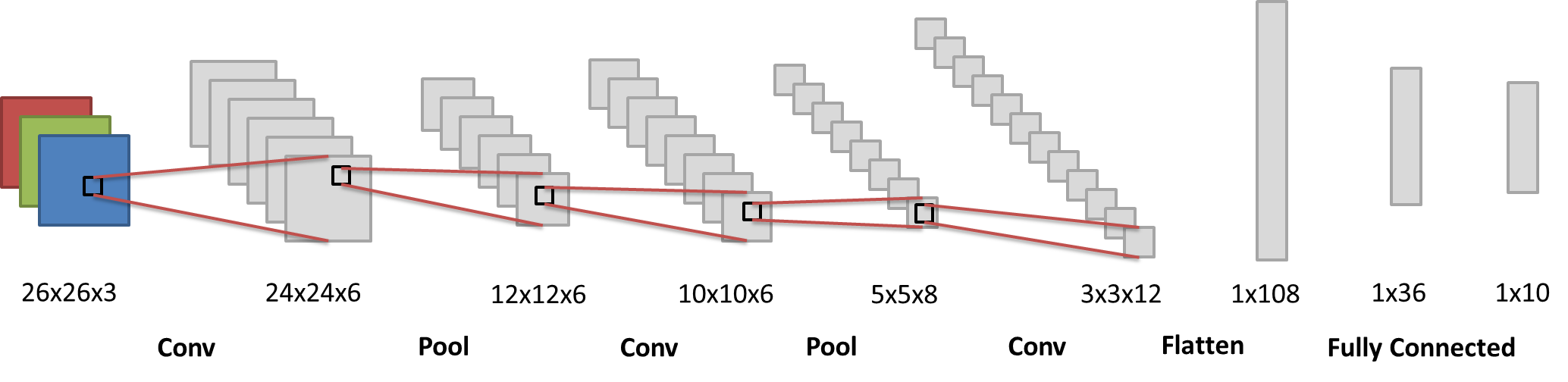
In the first step (Conv 26x26x3 -> 24x24x6), a 26x26x3 image are turned into a 24x24x6 image. The process is conducted by 6 (1) different (initialized by random) 3x3x3 (2) convolution kernels.

1. 6 kernels can generate 6 different 2D features (we usually regard the images in the middle process as features).
2. Note that the 3x3x3 is designed by (kernel width, kernel height, kernel channels). The 3x3x3 kernel is a 3D kernel to calculate convolution for each RGB channels of the original images respectively.

Then, the next step (Pool 24x24x6 -> 12x12x6), let us use a max-pool to illustrate the process. Pooling is the same as Subsampling, which, retrain only the representative such as the maximum in a kernel size matrix. It is clear to see that the image size is divided by the kernel size after applying the pooling.

In the previous diagram, we applied further convolution and pooling, which also follow the corresponding process. Finally, the 3x3x12 feature are flattened into a 1x108 linear layer of neurons, then they are connected to classical deep neural network, and a 10 classification results are shown in the output layer (1x10).

Conclusion

In this post, we have learned:

• The neural network can extract features from alternating the convolution kernel matrices in the back-propagation process by gradient descent.
• CNN layers are usually containing Convolution and Pooling to shrink the huge size of input neurons.
• After Convolution and Pooling, the features are usually flattened and connected to fully connected layers.
• The CNN architecture employs kenneling and subsampling to simplified the related neighborhood of pixels which could generate data redundancy.